Last week, I took my last class which is Neural Control of Movement. It was taught by professor Sara Solla who is a computational neuroscientist and it was about Generalized Linear Model (GLM) for neural data analysis. GLM is a very useful tool for both data scientists and neuroscientists (and also very popular). I think it’s a very good tool to have in mind. Sara taught GLM in from neuroscience perspective in a very intuitive way. I think that it would be nice to share some summarization of her lecture here.
Basic neural recording experimental set up
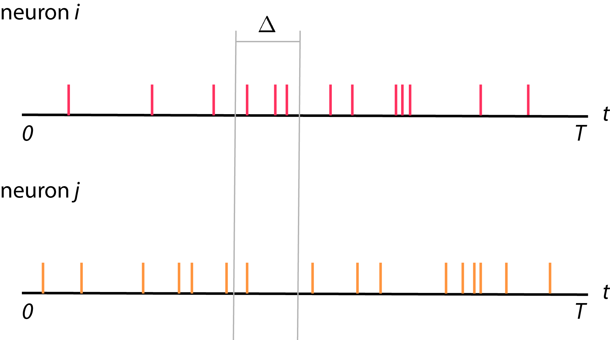
- So, let’s start from the simple set up. We will start from recording from two neurons
- \(i\) and \(j\) from time \(0\) to time \(T\) (see figure below).

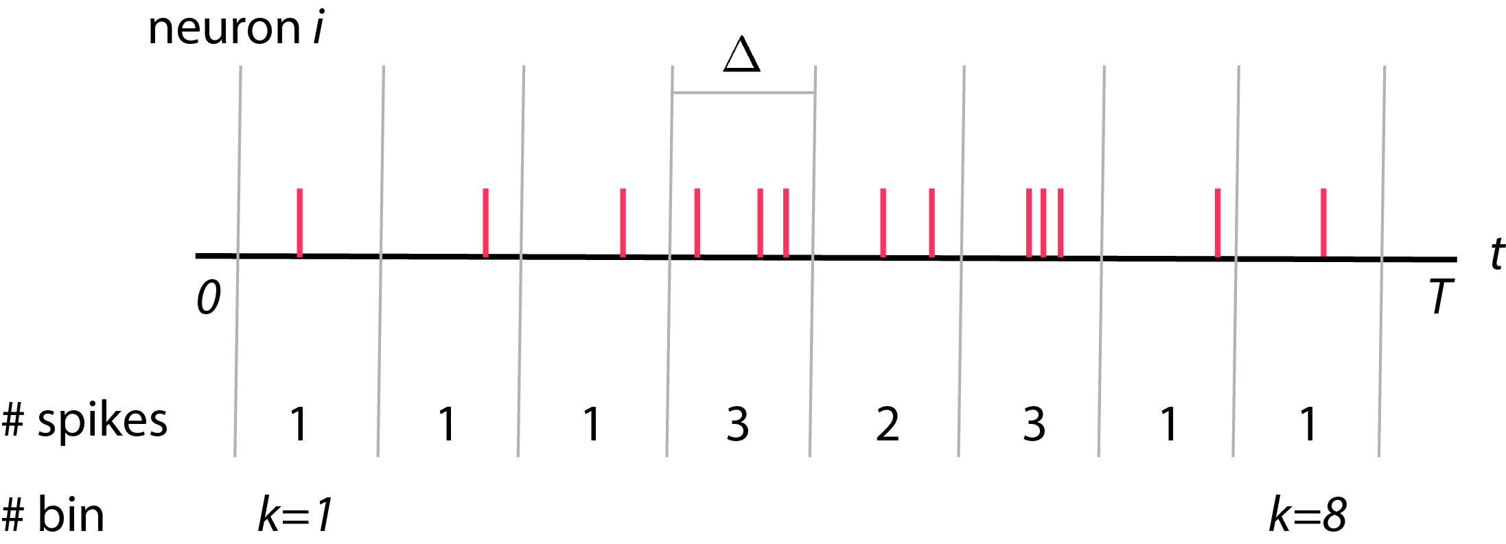
Typically, we record spike trains from neurons. We will then divide these spike trains recording into bins, each with size \(\Delta\). The total number of bins will be \(K\) where \(K = \frac{T}{\Delta}\). Each bins is indexed by \(k\), where \(1 \leq k \leq K\). Now, we will count number of spikes in each bins and call is as \(y_i (k)\) where \(y_i (k)\) is a spike count of neuron \(i\) in bin \(k\) (see figure below).
Let’s summarize what we’ve mentioned
- \(K = \frac{T}{\Delta}\) where \(K \) is total numbers of bins
- \(y_i (k)\) is number of spikes of neurons \(i\) in bin \(k\)
- \(y_i (k) = 0, 1, 2, \ldots \) which is non-negative integer
Before we are going forward, I would like to convince that \( y_i (k) \) is a random variable. That is, if we were to record exact same neuron in the same experimental set up, we won’t get the same spike counts as before. However, we assume that these neural spikes are drawn from some distribution with some statistic.
After the setup, what we want to do is we want to describe statistic of these activity i.e.
GOAL: Our goal is to describe expectation of \(y_i(k)\) or \(\langle y_i(k) \rangle \).
Formulation of (Poisson) Generalized Linear Model
Let’s make the set up more generalized where we record from \(N\) neurons and \(K\) bins.
\[\{ y_i (k)\}, 1 \leq i \leq N, 1 \leq k \leq K\]Assume number of spikes in each bin are drawn from poisson distribution with parameter \(\lambda\). Poisson distribution can be written as
\[p(y = n) = \frac{\lambda^n}{n!} e^{-\lambda}\]parameter of Poisson distribution is as follows
- mean of distribution: \(\langle y \rangle = \lambda\)
- variance: \( \sigma^2 = \langle y - \lambda \rangle^2 = \langle y^2 \rangle - \langle y \rangle^2 = \lambda \)
- Fano factor = \(\frac{variance}{mean} = \frac{\sigma^2}{\langle y \rangle} = \frac{\lambda}{\lambda} = 1 \)
As mentioned above, we want to construct GLM in order to describe all neurons \(i\) at all time bins \(k\). We can form the likelihood function from data as a product of all neurons and time bin
\[L = \prod_{i=1}^{N} \prod_{k=1}^{K} \bigg\{ \frac{\lambda_i(k)^{y_i(k)}}{y_i(k)!} e^{-\lambda_i(k)} \bigg\}\]Generally, what we do is take a log of likelihood (so called log-likelihood) which will turn all the product into summation
\[\begin{eqnarray} \ell &=& \ln L \nonumber \\ &=& \sum_{i=1}^{N} \sum_{k=1}^K \bigg\{ y_i(k) \ln \lambda_i (k) - \lambda_i(k) - \ln \big[ y_i(k)! \big] \bigg\} \nonumber \end{eqnarray}\]The beauty of this log-likelihood function is that each dimensions, we can show that the cost looks like concave downward. That is, we can minimize this cost function easily by gradient descent. You can see how we find gradient of log-likelihood function more in this tutorial from python library for GLM, pyglmnet.
Effect from other neurons
Now, we want to write down \(\lambda_i (k)\) in terms of effect from itself and other neurons (using some parameters \(\alpha_{ii}, \alpha_{ij}\)).
Activity of neuron \(i\) at bin \(k\) can be influenced from other neurons also. For example, effect of neural firing in dorsal or ventral premotor cortex area (PMd) from some time lag before can affect neural activity in primary motor cortex (M1). Theoretically, PMd might deal with some motion planning before M1 execute motor or movement task. In this case, we can formulate GLM consider effect of other neurons in the network to neuron \(i\). Suppose we consider some time lag from itself and other neurons until time \(\tau\)
\[\lambda_i (k) = \langle y_i (k) \rangle = \exp \big\{ \alpha_{i0} + \sum_{m=1}^{\tau} \alpha_{ii}(m) y_i (k - m) + \sum_{j=1, j \neq i}^{M} \alpha_{ij}(m) y_j (k - m) \big\}\]or we can sum all the activity from itself and from other neurons into one term,
\[\lambda_i (k) = \exp \big\{ \alpha_{i0} + \sum_{j=1}^N \sum_{m=1}^{\tau} \alpha_{ij}(m) y_j(k - m) \big\}\]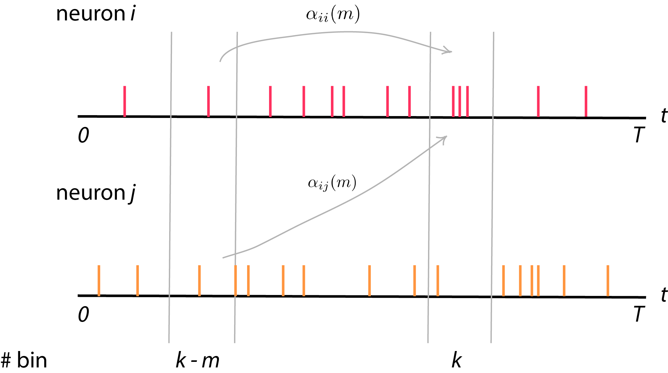
note that this can be called as linear-nonlinear model (L-NL) and this exponential function is one of link function from exponential family
we can again plug \( \lambda_i(k) \) to likelihood \(L\)
\[\begin{eqnarray} \ell &=& \ln L \nonumber \\ &=& \sum_{i=1}^{N} \sum_{k=1}^K \bigg\{ y_i (k) \Big[ \alpha_{i0} + \sum_{j=1}^{N} \sum_{m=1}^\tau \alpha_{ij}(m) y_j(k - m) \Big] \nonumber \\ && - \exp \Big[ \alpha_{i0} + \sum_{j=1}^{N} \sum_{m=1}^\tau \alpha_{ij}(m) y_j(k-m) \Big] - \ln \big[ y_i(k)! \big] \bigg\} \nonumber \end{eqnarray}\]If we looked through literature, these parameters sometimes claimed as effective connectivity. This means that in GLM, we cannot claim direct connectivity since neuron \(j\) might indirectly influence neuron \(i\) but we don’t actually know.
Connectivity in primary motor area (M1) and ventral premotor area (PMv)
One paper that analyze neural data using GLM was from Nature 2010 by Truccolo, Donoghue. Here, we want to find relationship of neural spikes between premotor area and motor area. We can again form GLM to describe activity in M1 area from both area M1 itself and PMv. We denote \(\lambda_i^{M}(k)\) and \(\lambda_i^{PM}(k)\) as neural activation in motor cortex and premotor cortex respectively. Activity in motor area can be model as follows:
\[\begin{eqnarray} \lambda_i^{M}(k) &=& \exp \big\{ \alpha_{i0} + \sum_{j=1}^{N_M} \sum_{m=1}^{\tau} \alpha_{ij}^{MM}(m) y_j^M(k-m) \nonumber \\ & & + \sum_{l=1}^{N_{PM}} \sum_{m=1}^{\tau} \alpha_{il}^{M-PM (m)} y_l^{PM} (k-m) \big\} \nonumber \end{eqnarray}\]Same in premotor area,
\[\begin{eqnarray} \lambda_i^{PM}(k) &=& \exp \bigg\{ \alpha_{i0} + \sum_{l=1}^{N_{PM}} \sum_{m=1}^{\tau} \alpha_{il}^{PM-PM}(m) y_j^{PM}(k-m) \nonumber \\ & & + \sum_{j=1}^{N_{M}} \sum_{m=1}^{\tau} \alpha_{ij}^{PM-PM (m)} y_j^{M} (k-m) \bigg\} \end{eqnarray}\]Not only neural activities from other areas that can be used in GLM. We can also incorporate effects from kinematics at some time lag \(m’\) too (with different time bin) i.e. (\(v_x(k + m’), v_y(k + m’)\) ). For example, we can add arm velocity in order to predict neural activity or neuron \(i\) at bin \(k\),
\[\begin{eqnarray} \lambda_i(k) &=& \exp \bigg\{ \alpha_{i0} + \sum_{m=1}^{\tau} \alpha_{ii}(m) y_i (k-m) + \sum_{j=1, j \neq i}^{M} \sum_{m=1}^{\tau} \alpha_{ij}(m) y_j(k-m) \nonumber \\ & & + \sum_{m'=0}^{\tau_K} \alpha_{ix}(m') v_x (k + m') + \sum_{m'=1}^{\tau_K} \alpha_{iy}(m') v_y (k + m') \bigg\} \end{eqnarray}\]If you see figure 1 from Truccolo, Donoghue, the parameters \(\alpha_{ii}\) and \(\alpha_{ij}\) are roughly as follows
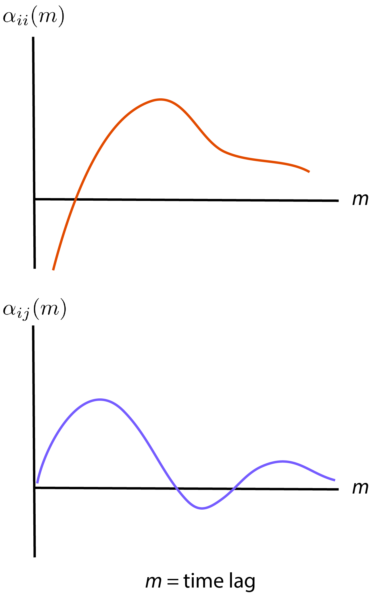
Basically, for neuron by itself, we will have some peak of parameter at some time lag (basically, the neuron has some refractory period of firing). And other neurons also influence by some time lag.
Where to start using GLM?
All the lecture above is mainly the formulation of GLM. However, it’s good to know how to derive gradient of GLM cost function also.
There are existing packages that implement Generalized Linear Model (GLM) and tutorial include:
In these packages, you can choose link function much more than poisson. In order to solve GLM cost function, past literatures use simple gradient descent algorithm or coordinate gradient descent algorithm which we won’t describe here.